Building a Bitemporal Index (part 3): Storage

And so here we are, the final part of the trilogy!

In the previous two parts, I’ve covered:

a taxonomy of bitemporal data - what does bitemporal data look like in practice?
'bitemporal resolution' - how we reconstruct the bitemporal history from fundamental events.

In part 2, I made a rather large hand-wavy assertion that:

On the write side, we could Just™ append events to the end of an append-only log
On the read side, we could assume that those events would be magically partitioned by entity-id, sorted by system-time descending, and easily filterable on common predicates.

The latter, in particular, is quite the assumption - rather a stretch to leave as 'an exercise for the reader'!

At this stage, it might seem magical - but as we’ll find out in this article, the truth is that it’s really just "good ol'-fashioned engineering". 😅

Before we start describing what XTDB does, though, let’s talk about the environment we’re working with:

XT’s high-level architecture

XTDB, by design, 'separates storage from compute' - indeed, this was one of the main aims we had for XT v2. We recognise that remote object storage (e.g. AWS’s 'S3', GCP’s 'Cloud Storage', Azure’s 'Blob Storage') is significantly cheaper than instance storage, and getting cheaper. With a 'database that remembers everything', this is critical in reducing the operational cost of an XT cluster.

An XT cluster consists of three distinct components:

A transaction log (e.g. Kafka): this gives us a total ordering of transactions - largely out of scope for this particular discussion but a core part of the system nonetheless.
Shared object storage: large, cheap, but remote.
Compute nodes: the work-horses. They have (ideally large) local caches, but are otherwise completely replaceable - the durability is provided by the two other components.

We owe this separation and focus on the shared log to Martin Kleppmann's 2015 talk, "turning the database inside-out", which very much inspired the design choice here.

Naturally, though, this comes with constraints:

The object storage being remote means that reads and writes are high-latency. For low-latency queries, we don’t want to be making reads of the object storage, so for this use-case it’s crucial to have decent size caches on the nodes themselves.

(Veterans of the software industry will immediately recognise this as one of our two hardest problems: cache invalidation, naming things, and off-by-one errors.)

Specifically:
- Object storage here prefers larger reads and writes - experimentally, we found it takes roughly the same time to download a 1-10MB file as it does for a 1-10kB file.
- It also rules out updating part of a file, as you might if you were maintaining files on a local disk.
- We can’t realistically rely on locking/co-ordinating updates to object-store files.
- We need to be aware of 'write amplification' - we don’t want, for example, to be shuffling lots of data around (as you might to rebalance a binary tree), because this will involve pulling multiple files down and uploading them all back up again.
Our decision to use Apache Arrow as the on-disk format imposes a similar constraint - these also cannot be updated in place (in general). Given our remote storage, this doesn’t actually add much marginal complexity - if we already cannot update-in-place, we may as well use the columnar benefits of Arrow!
The compute nodes don’t have any other inter-node communication except through the tx-log and object-store. This was largely a decision for simplicity - introducing communication here is not without its own complexity tradeoffs, things that can go awry.

(We may revisit this decision at some point, to reduce the dependency on Kafka - but, for now, it’s without a doubt helped us to get to this stage.)

So, two properties seem to fall out from these constraints: it makes sense that the files we upload to object storage be both immutable and deterministic. Immutable, because of the update-in-place characteristics; deterministic, because of the lack of communication between nodes - if two nodes upload the same file, we know that they have the same content.

With these constraints, two data structure spring to mind:

'hash array-mapped tries', or 'HAMTs'
'log-structure merge trees', or 'LSM' trees.

Let’s cover them in turn:

Hash Array-Mapped Tries - HAMTs

When XT nodes consume the transaction log, they temporarily store the bitemporal events from the newest transactions in an in-memory HAMT structure.

HAMTs were introduced by Phil Bagwell in his 2001 paper "Ideal Hash Trees", and have since become a cornerstone of persistent data structures in functional programming. Rich Hickey later popularized them through their use in Clojure’s immutable maps and sets.

The structure is simple but powerful: take the hash code of your key, split it into fixed-width segments (in Clojure: 5 bits for a branching factor of 2⁵ == 32; in XT, we use 2 bits for a branching factor of 4). Then, each level of your trie is an array, each cell representing one possible value of the hash prefix - e.g. we have four buckets: 00, 01, 10, and 11. At the leaves, we then have a page of data with the given hash prefix. When that leaf goes over a certain size threshold (1024, for us), we then split that leaf into another branching node.

Figure 1. A simple HAMT

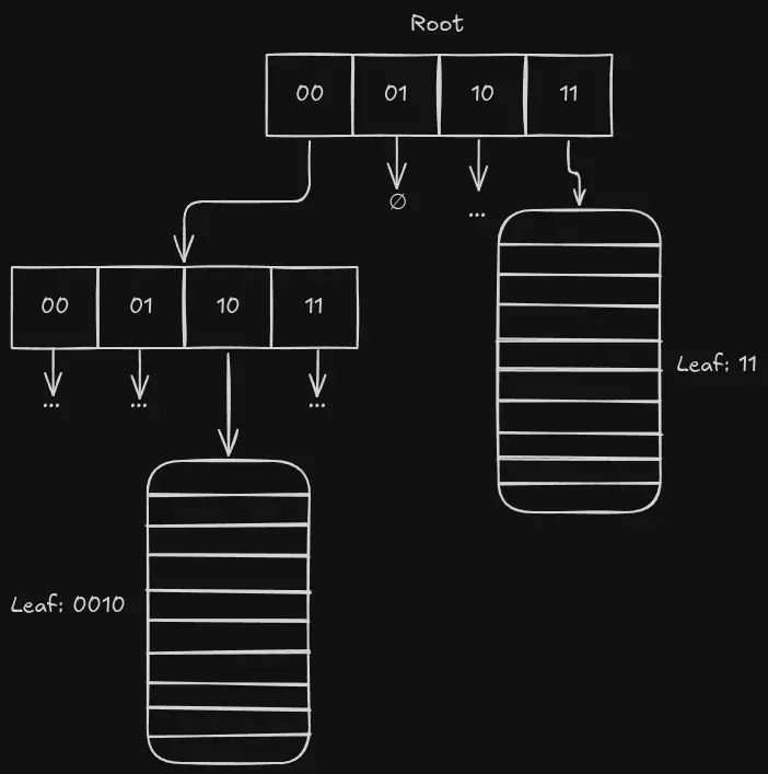
In XT, we use a 'hitchhiker tree' - a special kind of HAMT that’s more append-friendly by deferring the sorting within leaf nodes until they need to be promoted to a branch. The difference is beyond the scope of this article - I’d highly recommend David Greenberg’s excellent 2016 StrangeLoop talk, "Exotic Functional Data Structures".

After a number of transactions, this trie itself reaches a size threshold where we want to persist it to durable storage. We ensure that all of the leaves are sorted, then upload it to the object store, where it becomes the newest member of a shared LSM tree:

Log-Structured Merge Trees ('LSM' trees)

Let’s imagine what’d happen if we didn’t have LSM trees.

Let’s say over time we upload a hundred of these HAMTs. We could still run queries against these hundred files - they’re all individually sorted, first by entity-id, then by system-time - so we can perform the bitemporal resolution process to serve queries by merge-sorting the related pages of each of the files.

However, this clearly doesn’t scale - the more files you add, the more inputs you have in your merge-sort. Even if you want to find a single value, you have to look in every L0 to see whether there are any relevant events.

Act 1: Compaction

So, we call these files 'level 0', or 'L0' files, and start a background process to combine these files together - 'compaction'.

When we reach a certain number of L0 files, a compaction process on one of the nodes merge-sorts them together into a level 1 ('L1') file, so that we don’t have to redo this work on every query. Once this L1 file’s been written, the L0 files are considered 'superseded' - we don’t need to read from these any more.

In a normal LSM tree (in a mutable database, say), the implementors will likely take this opportunity to combine updates for a given key. If I set x = 4, then later set x = 5, these two updates eventually end up in the same LSM tree file, at which point they drop the earlier update. XT, though, is 'the database that remembers everything'! So, for us, this operation is a 'concat' - when we compact, we concatenate all of the bitemporal events so that we can use any of them in across-time queries.

What happens when L1 becomes full, I hear you say? Well, it’s "turtles all the way down" - we compact L1s into L2s, and so on!

This is the essence of a log-structured merge tree (LSM tree):

Data is ingested quickly into small, sorted batches.
These batches are later merged into larger, coarser-grained levels.
Old data naturally migrates to deeper levels, where it becomes more compact, more stable, and less frequently accessed.

This works beautifully with our constraints:

Writes are batched and append-only.
Files are immutable, with a well-defined definition for when they’re superseded - this greatly simplifies local cache invalidation.
Compaction is a background task, and there are enough fine-grained tasks for the nodes to not require co-ordination in practice.
We publish metadata for each file - the min/max values for numeric columns, bloom filters for non-numerics - so that we can quickly rule out needing to scan as many files as possible.

Naively compacting a handful of L1s into L2s, a handful of L2s into L3s and so on, though, would result in larger and larger files as you go through the levels.

Act 2: Sharding

You’ll recall, though, that the individual files in our LSM tree contain HAMTs - data structures that partition the events by a prefix of their key.

This gives us a great opportunity to re-use this partitioning - albeit this time at the level of whole files, rather than pages within a file.

So, when we go from L1 to L2, rather than compacting four L1s into one L2, we instead compact four L1s into four L2s. The first compaction task filters it to events with a 00 bit prefix, the second 01, the third 10 and the fourth 11. When the fourth L2 file is written, we then consider the L1 files 'superseded', and the L2 files 'live'.

At deeper levels, we apply the same pattern as we did in the in-memory HAMTs, just using more of the prefix. L3 → L4, for example, uses three segments of entity-id, so four L3 files with prefix 21 become four L4 files with prefixes 210, 211, 212 and 213.

This has a few nice properties:

By compacting four files into four files, the files themselves remain roughly equivalently sized - we target 100MB, for example.
By making the compaction tasks more fine-grained, we give compute nodes more compaction work to choose from, so there’s less chance of them choosing the same tasks.

(It doesn’t really matter if they do - the process is deterministic, so they’ll all arrive at the same answers - just that it’s duplicated work.)
Given one of the most common low-latency queries is to look up a document by primary key, we can now very quickly rule out whole shards of the key-space.

That said, though: by partitioning by ID alone we eventually end up shuffling all of the history for each entity together - queries still need to sift through all of this history to figure out the current state (one of the key query categories in part one). Not a problem if each entity only has a handful of updates (i.e. in the user-profile case) - but when one of your early Design Partners suggests they want to use XTDB to store sensor data, where each entity has hundreds of thousands of versions, it’s back to the whiteboard! ^[1]

Act 3: 'Recency'

I think I’d better think it out again!

— Fagin
"Reviewing the Situation", Oliver!

In 2.0.0-beta7 we re-sharded the XTDB primary index, introducing the concept of 'recency'.

Initially in the 2.x line we used a k-d tree to store the temporal information, with six dimensions: four temporal (valid-from, valid-to, system-from, system-to), and two content (entity-id, entity-version). Unfortunately, this wasn’t as performant as we needed to either update or query - for as-of-now queries, for example, you cannot filter on three of those six dimensions. Having six dimensions is also not particularly practical if you’re looking to partition your data.

After some analysis, I defined a heuristic I called 'recency' - a means of collapsing the temporal dimensions into one, while still preserving the selectivity properties we needed in the most common cases.

recency (of a version)

the maximum timestamp T for which the row was believed valid for both valid-time = T and system-time = T

In pictures:

For a superseded bitemporal event (i.e. where there’s a later update) its period of validity tends to look like an 'L' shape. We calculate recency by looking at the VT = ST line, and choosing the 'last point within the polygon':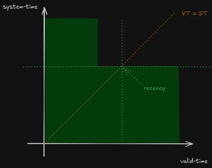

Figure 2. Calculating recency
We then know that no query with valid-time/system-time filters above or to the right of the recency can possibly be influenced by this event:

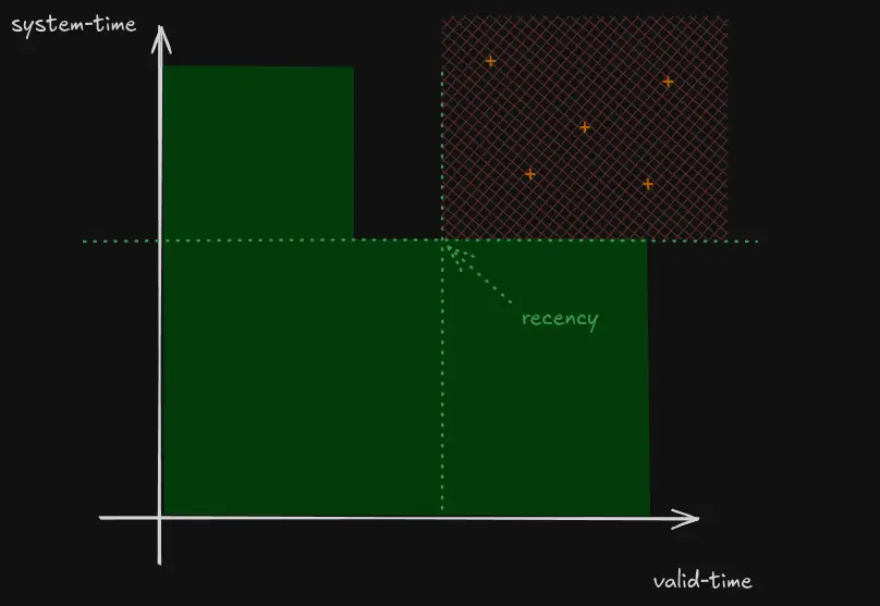Figure 3. Queries unaffected by this document version (+)

As a heuristic, recency is permitted to be an over-estimate, but never an under-estimate. This means that we can group rows with a similar recency together (into a file, say) and then use the maximum recency from all of the rows as the recency for the file as a whole. If a query is only interested in data more recent than that recency (especially in the most common 'as of now' case), we can elide the whole file from our scan!

Having reduced the sharding dimensions significantly to just entity-id and recency, we needed to decide what this sharding should look like in practice.

Act 4: the 'Lindy Effect'

The 'Lindy effect' theorises that:

the future life expectancy of non-perishable things is proportional to their current age.

While there are obviously exceptions, it broadly holds true in many domains:

Business: the older a company is, the more likely it is to survive into the future.
Books: the longer they’ve been in print, the more likely they’ll continue to be in print.
Music: similarly - especially as "they don’t make records like they used to".

Closer to home:

Garbage collection: generational garbage collections will compact newer objects much more frequently than older objects on the assumption that newer objects are used for a short period of time then discarded; older objects are more likely to be required throughout the lifetime of the application.

Most importantly to us, though:

Data systems: newer data is much more likely to be superseded than data that has already remained current for a long period of time.

Looking back to the taxonomy in part one, we see this principle holding in the various use-cases:

User profiles: not often updated, versions stay current for a long time.
Trades/orders: after an initial period of updates, the final state remains valid indefinitely.
Sensor readings/market pricing: probably superseded before you get to the end of this sentence.

We make use this principle in XTDB by splitting the LSM tree at level 1. After level 1, a document version can take one of two paths: the survivor or the historical. ^[2] The current partition is then sharded solely by entity-id, as before; the historical partition is first partitioned by recency - the time at which the row was superseded.

In practice, for any given table, it looks something like this:

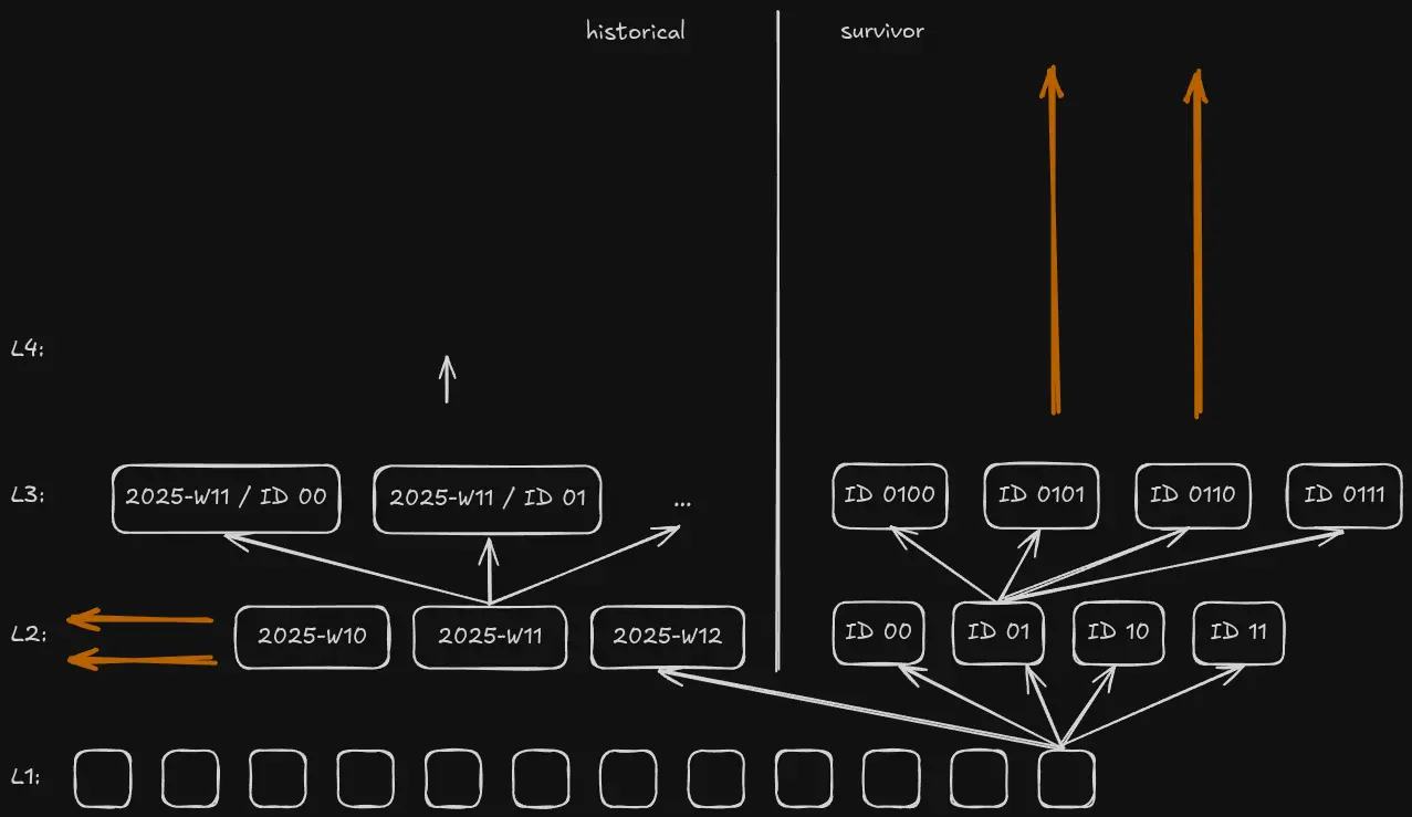
This diagram shows the fully general case but, realistically, data for any individual entity type will usually only grow significantly in one of the two dimensions:

User profiles: unless the versions get superseded quickly, they’ll likely make it to the survivor side (even the ones that are later superseded). Given the cardinality (number of distinct user profiles), the survivor side will likely grow deep; the historical side will likely be relatively small.
Trades/orders: the temporary initial states will go into historical; the final states will go into survivor.
Sensor readings/market pricing: given the cardinality (number of distinct sensors/stock tickers) the historical section likely won’t grow that deep, but it’ll certainly be very wide. (The 'survivor' section is non-existent in this case.)

As a heuristic, it absolutely doesn’t have to be a perfect split - some historical versions may make it into the survivor side - the important thing is that it works plenty well enough in enough cases!

Wrapping up

All of which brings us to a state where we have a shared, sharded, sorted index of bitemporal events in cheap, reliable storage, collaboratively maintained by a group of independent compute nodes!

If you’ve enjoyed this deep-dive series as much as I’ve enjoyed writing it, please do let us know - come join us in the comments, or get in touch at hello@xtdb.com!

James

P.S. and, oh, btw - do keep an eye out for our 2.0.0 launch announcement 😁

1. I jest, of course, I’m genuinely really grateful for this requirement - XT is in a much better place as a result 🙏

2. We assume that if a row is going to be superseded, it will have been superseded by the time it leaves L1. In practice, this seems to work enough of the time to be a useful rule!