Building a Bitemporal Index (part 2): "Bitemporal Resolution"

Last week I wrote a taxonomy of bitemporal data - identifying different shapes of bitemporal data and queries.

This time, we’re starting to look at how XTDB, through a built-in understanding of how temporal data works in practice, handles this data more efficiently than a regular relational database.

First, let’s run through how a naïve implementation might approach a bitemporal table, and appreciate why bitemporality has the (IMO, unfair) reputation for 'always introducing complexity':

The destination

In XTDB, we very much embrace the idea of the 'Epochal Time Model', from Clojure author Rick Hickey’s 2009 talk, "Are We There Yet?":

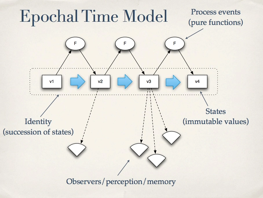
The fundamental idea here is that an 'identity' is a mutable pointer to one of a series of individual state values. Processes (functions) are applied atomically to the current state and return a new state. Observers then dereference/snapshot these pointers, to work with an immutable value - regardless of what other concurrent updates are happening, observers see a single, consistent state of the world.

In XTDB, inspired by Datomic before it, this same philosophy applies to entities in the database. Indeed, Rich himself coined and popularised the phrase "Database as a Value" through his 2012 talk of the same name - the database as a whole being a series of immutable values; each transaction applied as a pure function from one database value to the next. Querying users are then able to take a snapshot of any one of these database versions, running multiple queries against the same consistent snapshot.

I vividly remember this talk landing. Even amongst Rich’s back catalogue, I don’t think it’s an exaggeration to call this one 'revolutionary' - applying the simple state model of Clojure to a whole database.

Datomic is 'unitemporal' - it manages 'system' (a.k.a. 'transaction') time on behalf of the user, each entity having a single timeline of immutable values through system time. XTDB’s bitemporality adds an extra dimension to this: 'valid time' (a.k.a. 'business time', 'application time' or 'domain time' - three cheers for consistent naming in our industry!).

Valid time is essential for use cases when the time where facts become true/false doesn’t necessarily line up with when the system finds out about them - and even more so when auditors are involved!

So, at any one system time, rather than a single value, each XTDB entity has a whole timeline.

Let’s play it through, for a single entity:

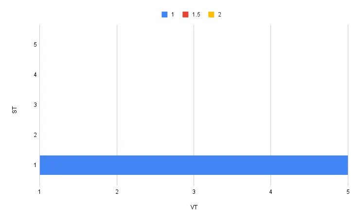
At time T1, we add a new document at version 1. At this point, we believe that the version will always be 1 ('until corrected'):
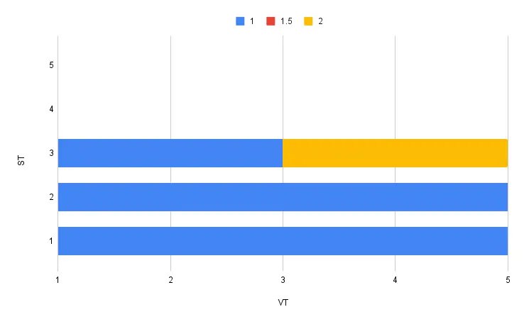
At time T3, we then update this document to version 2. The timelines for system-time T1 and T2 remain unaltered; at T3, we now know that the document was version 1 until T3 and version 2 afterwards.
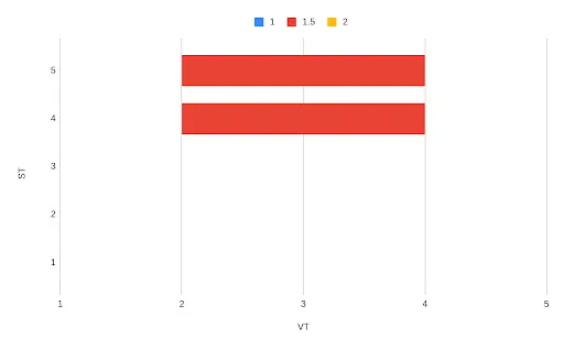
At time T4, we realise that we missed an update: that, from (valid) time T2 to T4 the document should have been at version 1.5. Again, the previous timelines are unaltered; now, we add another timeline:

At any point, observers querying XTDB can take an immutable snapshot of the whole database (choosing a point in system time). There they see the valid-time history for each entity, as the system knew it at that point in time.

Here, it becomes clear why valid time is essential for audit-heavy use cases. Let’s say an auditor asks you to justify a decision that you made at time T3 - you can reliably demonstrate that even though you now know that the value is 1.5 at (valid) time T3, that’s not the data you had available at (system) time T3; that’s not the data that you based your decision on.

"How not to do it":

The traditional approach here, in normal relational databases, is to add four extra columns to tables you want to be bitemporal: valid-from, valid-to, system-from and system-to.

These then need to be maintained on every insert, update and delete - often achieved through triggers, sometimes (!) manually.

Let’s see what that involves:

Add document at T1, version = 1:

system_time valid_time version

T1 → ∞

T1 → ∞

1
Update document at T3, version = 2:

system_time valid_time version

T1 → T3

T1 → ∞

1

T3 → ∞

T1 → T3

1

T3 → ∞

T3 → ∞

2

Here we have to modify the original row to 'close out' the system-time for valid-time T1 → ∞ (system past, valid current), add another historical row (system current, valid past), and then add the new row. Whew.
At T4, correct document from T2 → T4, version = 1.5:

system_time valid_time version

T1 → T3

T1 → ∞

1

T3 → T4

T1 → T3

1

T3 → T4

T3 → ∞

2

T4 → ∞

T1 → T2

1

T4 → ∞

T2 → T4

1.5

T4 → ∞

T4 → ∞

2

This one’s a doozy - even after however-many years experience working on a bitemporal database, I’m sure you’ll believe me when I say it took me a few goes to get this one right 😅.

system_time	valid_time	version
T1 → ∞	T1 → ∞	1

system_time	valid_time	version
T1 → T3	T1 → ∞	1
T3 → ∞	T1 → T3	1
T3 → ∞	T3 → ∞	2

system_time	valid_time	version
T1 → T3	T1 → ∞	1
T3 → T4	T1 → T3	1
T3 → T4	T3 → ∞	2
T4 → ∞	T1 → T2	1
T4 → ∞	T2 → T4	1.5
T4 → ∞	T4 → ∞	2

Don’t do this by hand, folks!

Quite aside from the complexity, it also doesn’t tend to perform well:

On insert, the database is having to both read and write to many unrelated rows.
You have a 2x 'storage amplification' - you’re storing each row twice.
You now have to consider how best to index this table - what columns to include in the index? In what order?
When you query the data, you have a lot of historical data to filter out.

Or, you could choose a database that’s been built with this understanding baked in from Day One.

Introducing "bitemporal resolution"

XT, of course, doesn’t do it like this - either on the write or read side.

On the write side, we do the quickest thing possible - adding a single row to an append-only log. In this log, alongside the document, we store valid-from/valid-to and system-from - N.B. not system-to, for reasons that we’ll cover in a bit.

Table 1. XT’s append-only event log ^[1]
system_from	valid_time	version
T1	T1 → ∞	1
T3	T3 → ∞	2
T4	T2 → T4	1.5

This is the minimal form of bitemporal data - exactly what the incoming transactions specify, and no more.

When we come to read this data, we perform a process similar to event sourcing - playing through the history - but in reverse system-time order.

Why reverse?

Well, if we played it forward we’d have to do exactly the same algorithm as above, but just at query time instead, which would still be slow - thanks for coming to my TED talk 🙂.

A few observations, before we run through the bitemporal resolution algorithm:

For as-of-now queries (the most common, by a country mile), we can terminate as soon as we see the relevant entry - events earlier in system-time cannot supersede later events for the valid-time period in the later event.

So if I’m playing backwards through the above table at time T5, I:

read and discard the third row - it’s outside my valid-time
read the second row, notice that it covers the time I’m interested in
skip reading any other historical rows

For back-in-time queries, we can skip over later events - events are never visible earlier than their system-from, nor outside of their valid-time period.

Let’s say I query for time T1 - I can very quickly skip rows 3 and 2.
Queries that don’t project the four temporal columns don’t need to calculate them - they only need to ascertain whether each event is visible to the given query or not.

Full bitemporal materialization

As you can see, for most queries, there’s already a fair few optimisations that mean we don’t need to do as much work as the naive implementation.

Taking the worst case, though, let’s say we’re asked to materialize the full bitemporal state of the table.

We play it backwards:

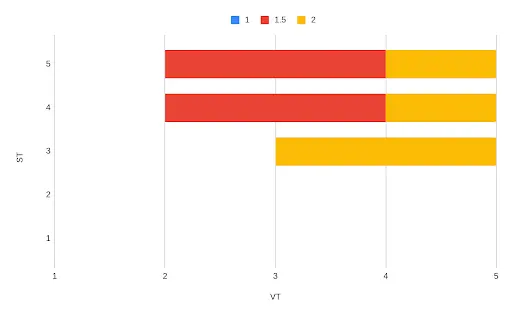
At T4, for T2 → T4, version = 1.5:

system_time valid_time version

T4 → ∞

T2 → T4

1.5
We now additionally maintain a data structure we call the 'ceiling': for each interval in valid-time, this keeps track of the latest system-time we haven’t yet covered in processed events.

In this example, the ceiling is currently infinite outside of the range we’ve specified, and capped at T4 between T2 and T4:

valid_time ceiling (system_time)

-∞ → T2

∞

T2 → T4

T4

T4 → ∞

∞
Applying the next event (backwards in time): at T3, version = 2.

Looking at the ceiling, we see that this event overlaps two of the intervals. We therefore need two rows added to our result:

system_time valid_time version

T4 → ∞

T2 → T4

1.5

T3 → T4

T3 → T4

2

T3 → ∞

T4 → ∞

2
Let’s update the ceiling - the event has brought the ceiling down for T3 → ∞:

valid_time ceiling (system_time)

-∞ → T2

∞

T2 → T3

T4

T3 → ∞

T3
Finally, at T1, insert version 1.

Again, we look at the ceiling and see that our event overlaps three intervals, so we add three rows:

system_time valid_time version

T4 → ∞

T2 → T4

1.5

T3 → T4

T3 → T4

2

T3 → ∞

T4 → ∞

2

T1 → ∞

T1 → T2

1

T1 → T4

T2 → T3

1

T1 → T3

T3 → ∞

1

system_time	valid_time	version
T4 → ∞	T2 → T4	1.5

valid_time	ceiling (system_time)
-∞ → T2	∞
T2 → T4	T4
T4 → ∞	∞

system_time	valid_time	version
T4 → ∞	T2 → T4	1.5
T3 → T4	T3 → T4	2
T3 → ∞	T4 → ∞	2

valid_time	ceiling (system_time)
-∞ → T2	∞
T2 → T3	T4
T3 → ∞	T3

system_time	valid_time	version
T4 → ∞	T2 → T4	1.5
T3 → T4	T3 → T4	2
T3 → ∞	T4 → ∞	2
T1 → ∞	T1 → T2	1
T1 → T4	T2 → T3	1
T1 → T3	T3 → ∞	1

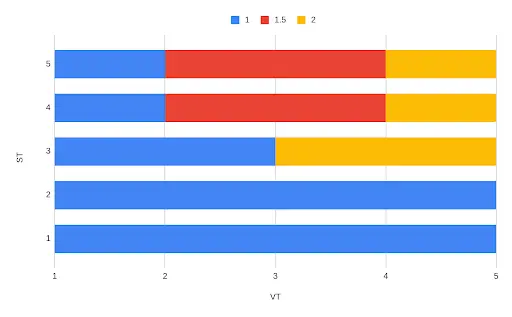
Notice that:

We’ve ended up at the same result - well, you’d have been disappointed if we didn’t!
More importantly, though: at no point have we had to either look at or modify rows added in previous events. This means that we can stream the rows out as soon as we calculate them, and we don’t need to keep them in memory.
We’ve only stored each row version once.

What’s next?

The more skeptical readers will have noticed that I’ve glossed over a couple of details here.

Particularly, I’ve made a big assumption here that we have all of the events in the system available to us, partitioned by entity ID, sorted by system-time, for every query. In XT, to complicate things further, this data may well live on remote object storage (because the storage is independent of the compute nodes). Downloading and reading all of that data obviously isn’t practical, so there’s plenty more we still need to do to make this a performant database.

In part 3, we’ll cover how we index these events in remote storage in order to execute these queries efficiently - stay tuned!

In the meantime, please do come join us in the comments - we’d love to hear from you.

James

1. This log is distinct from the Kafka log that we submit transactions to - this is a data structure that we store in the object-store.