SQL pipelines: reducing some of the accidental structure in SQL

Recently, the SQL innovation-du-jour seems to be to add 'pipeline' syntax:

Google added it to BigQuery from last October (becoming the default in February of this year).
Databricks announced its addition last week.

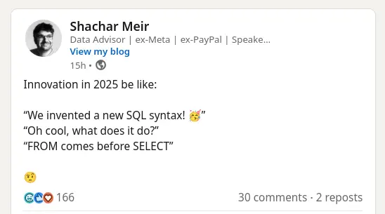
It’s even started attracting satire on LinkedIn:

I completely agree with the rationale behind pipelining:

It does more closely mirror the evaluation order of the underlying relational algebra. IMO, that’s not reason enough on its own, because knowing where to look is second nature to an engineer familiar with SQL (of which there are many in our industry).
It makes SQL queries more composable: you can incrementally build and test queries - uncomment one operator at a time to check where your query’s breaking.
It does reduce the amount of subqueries you need to express more complex SQL queries.

That said, I believe they’ve both missed a trick - a place on the solution spectrum that’s less of a deviation from the original SQL, but still yields these benefits.

You don’t need to add any more syntactic operators to SQL in order to be able to re-order (certain) clauses. In XTDB, the SQL pipelining that we released in January (in order to bring over some of the benefits of XTQL to our SQL users) doesn’t require any new syntax.

The trick is realising how SQL operators can affect each other. By and large, the operators themselves form a pipeline … almost - it’s the exceptions to the rule that cause the complexity.

A trip into the SQL spec

(feel free to skip this section if you just want to see how it works in XTDB)

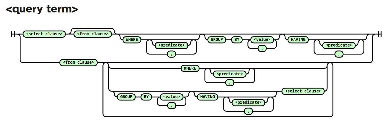
For example, the SQL spec says that every query ^[1] starts evaluation from the FROM clause.

The FROM clause already evaluates pretty much linearly. It’s a sequence of 'table references' (e.g. FROM <table-ref-1>, <table-ref-2>, …)

A table reference can itself be:

a base table: FROM foo
a table sub-query: FROM (SELECT … FROM foo)
a 'lateral' sub-query: FROM foo, LATERAL (SELECT … FROM bar WHERE bar.id = foo.bar_id)
a join (defined recursively): FROM (left-table-ref JOIN right-table-ref).

Contrary to popular belief, JOIN is not a top-level SQL construct - it lives within FROM - so FROM a, b JOIN c JOIN d is bracketed:
```
FROM (a CROSS JOIN ((b JOIN c) JOIN d))
```
So, if you see me pedantically indenting SQL like this:
```
SELECT ...
FROM a
  JOIN b ON (...)
  JOIN c ON (...)
WHERE ...
```
i.e. indenting the JOIN beyond the FROM - that’s why!

After the FROM/JOIN clauses, WHERE, GROUP BY and HAVING apply linearly, and finally, SELECT.

ORDER BY is an interesting one: in a 'simple query' (without any UNION, INTERSECT or EXCEPT), ORDER BY mostly runs after the SELECT - any columns that are created in the SELECT are visible to the ORDER BY. But (through what the spec calls 'extended order by clauses'), it is allowed to read values from before the SELECT clause projects them away - i.e. it appears to run both before and after the SELECT. A fun one to implement in our SQL compiler, safe to say!

Sub-queries

If you need any other structure, you’ll need to use sub-queries.

I’ve written previously at length about these: "The missing SQL sub-queries" - so I’ll elide that conversation here.

Pipelining without the pipes

In XTDB, we use the existing constructs in SQL to achieve the same thing.

A railroad diagram showing the top-level structure of an XTDB SQL query

Figure 1. for those who enjoy railroad diagrams: the top is standard SQL; the bottom is XTDB’s extension.

In addition to standard ordering (because heaven knows there are enough people and tools that are familiar with it) we also allow the following:

FROM/JOIN
Then, any number of 'tails' - either:
- WHERE
- (optionally) GROUP BY, (optionally) HAVING, SELECT
Finally, ORDER BY - we exclude this from the pipelining due to the complexities outlined above.

These tails then transform neatly into unary relational algebra operators for execution.

Some examples:

Example 1: a frequency distribution

-- in standard SQL: a sub-query
SELECT order_count, COUNT(*) AS freq          -- (5)
FROM (
  SELECT customer_id, COUNT(*) AS order_count -- (3)
  FROM orders                                 -- (1)
  GROUP BY customer_id                        -- (2)
) order_counts
GROUP BY order_count                          -- (4)
ORDER BY order_count DESC                     -- (6)

-- XTDB (take 1):
FROM orders                                   -- (1)
GROUP BY customer_id                          -- (2)
SELECT customer_id, COUNT(*) AS order_count   -- (3)
GROUP BY order_count                          -- (4)
SELECT order_count, COUNT(*) AS freq          -- (5)
ORDER BY order_count DESC                     -- (6)

-- XTDB (take 2 - because we can omit `GROUP BY` in this case)
FROM orders
SELECT customer_id, COUNT(*) AS order_count
SELECT order_count, COUNT(*) AS freq
ORDER BY order_count DESC

Example 2: filtering by the results of a window function - select the top 5 posts of each author

-- in standard SQL: again, a sub-query
SELECT *                                                                       -- (5)
FROM (
  SELECT p.title, like_count,                                                  -- (3)
         ROW_NUMBER () OVER (PARTITION BY author_id ORDER BY like_count DESC) idx
  FROM posts p                                                                 -- (1)
  WHERE author_id IN ('james', 'jeremy', ...)                                  -- (2)
)
WHERE idx <= 5                                                                 -- (4)

-- XTDB
FROM posts p                                                                   -- (1)
WHERE author_id IN ('james', 'jeremy', ...)                                    -- (2)
SELECT p.title, like_count,                                                    -- (3)
       ROW_NUMBER () OVER (PARTITION BY author_id ORDER BY like_count DESC) idx
WHERE idx <= 5 -- N.B. WHERE applied after SELECT                              -- (4)
-- also no final `SELECT` needed here

In our experience, we also find that AI tools are perfectly capable of understanding and generating SQL in this order - well, it’s something you have to check in this day and age!

Let us know what you think!

Would you choose to write SQL this way?

Have we missed a trick?

Please do join us in the comments!

James

Appendix: TPC-H

TPC-H is a well-known OLAP benchmark to compare the performance of various databases. It models a wholesale supplier’s business, focusing on managing, selling, and distributing products, and includes domains like customers, orders, parts, suppliers, and shipping.

Here we translate some of the 22 queries into pipeline format for your perusal:

Q1: "Pricing Summary Report Query - reports the amount of business that was billed, shipped, and returned"

-- standard
SELECT
  l_returnflag,
  l_linestatus,
  SUM(l_quantity) AS sum_qty,
  ...
  COUNT(*) AS count_order
FROM lineitem AS l
WHERE l_shipdate <= DATE '1998-12-01' - INTERVAL '90' DAY
GROUP BY l_returnflag, l_linestatus
ORDER BY l_returnflag, l_linestatus

-- XTDB
FROM lineitem AS l
WHERE l_shipdate <= DATE '1998-12-01' - INTERVAL '90' DAY
SELECT
  l_returnflag,
  l_linestatus,
  SUM(l_quantity) AS sum_qty,
  ...
  COUNT(*) AS count_order
ORDER BY l_returnflag, l_linestatus

Q7: "Volume Shipping Query - determines the value of goods shipped between certain nations to help in the re-negotiation of shipping contracts."

-- standard
SELECT supp_nation, cust_nation, l_year,
       SUM(volume) AS revenue
FROM (
  SELECT
    n1.n_name                              AS supp_nation,
    n2.n_name                              AS cust_nation,
    EXTRACT(YEAR FROM l.l_shipdate)        AS l_year,
    l.l_extendedprice * (1 - l.l_discount) AS volume
  FROM
    supplier AS s,
    lineitem AS l,
    orders AS o,
    customer AS c,
    nation AS n1,
    nation AS n2
  WHERE
    s.s_suppkey = l.l_suppkey
    AND o.o_orderkey = l.l_orderkey
    AND c.c_custkey = o.o_custkey
    AND s.s_nationkey = n1.n_nationkey
    AND c.c_nationkey = n2.n_nationkey
    AND (
      (n1.n_name = 'FRANCE' AND n2.n_name = 'GERMANY')
      OR (n1.n_name = 'GERMANY' AND n2.n_name = 'FRANCE')
    )
    AND l.l_shipdate BETWEEN DATE '1995-01-01' AND DATE '1996-12-31'
) AS shipping

GROUP BY supp_nation, cust_nation, l_year
ORDER BY supp_nation, cust_nation, l_year

-- XTDB
FROM
  supplier AS s,
  lineitem AS l,
  orders AS o,
  customer AS c,
  nation AS n1,
  nation AS n2
WHERE
  s.s_suppkey = l.l_suppkey
  AND o.o_orderkey = l.l_orderkey
  AND c.c_custkey = o.o_custkey
  AND s.s_nationkey = n1.n_nationkey
  AND c.c_nationkey = n2.n_nationkey
  AND (
    (n1.n_name = 'FRANCE' AND n2.n_name = 'GERMANY')
    OR (n1.n_name = 'GERMANY' AND n2.n_name = 'FRANCE')
  )
  AND l.l_shipdate BETWEEN DATE '1995-01-01' AND DATE '1996-12-31'
SELECT
  n1.n_name                              AS supp_nation,
  n2.n_name                              AS cust_nation,
  EXTRACT(YEAR FROM l.l_shipdate)        AS l_year,
  l.l_extendedprice * (1 - l.l_discount) AS volume

SELECT supp_nation, cust_nation, l_year,
       SUM(volume) AS revenue

ORDER BY supp_nation, cust_nation, l_year

Q13: "Customer Distribution Query - seeks relationships between customers and the size of their orders"

-- standard
SELECT c_orders.c_count, COUNT(*) AS custdist
FROM (
  SELECT c.c_custkey, COUNT(o.o_orderkey)
  FROM
    customer AS c
    LEFT JOIN orders AS o
      ON c.c_custkey = o.o_custkey AND o.o_comment NOT LIKE '%special%requests%'
  GROUP BY c.c_custkey
) AS c_orders (c_custkey, c_count)
GROUP BY c_orders.c_count
ORDER BY custdist DESC, c_orders.c_count DESC

-- XTDB
FROM customer AS c
  LEFT JOIN orders AS o
    ON c.c_custkey = o.o_custkey AND o.o_comment NOT LIKE '%special%requests%'
SELECT c.c_custkey, COUNT(o.o_orderkey) AS c_count
SELECT c_count, COUNT(*) AS custdist
ORDER BY custdist DESC, c_count DESC

Q22: "Global Sales Opportunity Query - identifies geographies where there are customers who may be likely to make a purchase"

-- standard
SELECT
  custsale.cntrycode,
  COUNT(*)                AS numcust,
  SUM(custsale.c_acctbal) AS totacctbal
FROM (
  SELECT SUBSTRING(c.c_phone FROM 1 FOR 2) AS cntrycode, c.c_acctbal
  FROM customer AS c
  WHERE
    SUBSTRING(c.c_phone FROM 1 FOR 2) IN ('13', '31', '23', '29', '30', '18', '17')
    AND c.c_acctbal > (
      SELECT AVG(c.c_acctbal)
      FROM customer AS c
      WHERE c.c_acctbal > 0.00
        AND SUBSTRING(c.c_phone FROM 1 FOR 2) IN
            ('13', '31', '23', '29', '30', '18', '17')
    )
    AND NOT EXISTS(
      SELECT *
      FROM orders AS o
      WHERE o.o_custkey = c.c_custkey
    )
) AS custsale
GROUP BY cntrycode
ORDER BY cntrycode

-- XTDB
FROM customer AS c

WHERE
  SUBSTRING(c.c_phone FROM 1 FOR 2) IN ('13', '31', '23', '29', '30', '18', '17')
  AND c.c_acctbal > (
    FROM customer AS c
    WHERE c.c_acctbal > 0.00
      AND SUBSTRING(c.c_phone FROM 1 FOR 2) IN
          ('13', '31', '23', '29', '30', '18', '17')
    SELECT AVG(c.c_acctbal)
  )
  AND NOT EXISTS(
    FROM orders AS o
    WHERE o.o_custkey = c.c_custkey
  )

SELECT SUBSTRING(c.c_phone FROM 1 FOR 2) AS cntrycode, c.c_acctbal

SELECT cntrycode, COUNT(*) AS numcust, SUM(c_acctbal) AS totacctbal

ORDER BY cntrycode

1. putting aside CTEs for a moment