Tuesday, 23 July, 2024
Taking the ² out of O(n²)
 James Henderson
 A few days ago we noticed a significant slow-down in XTDB 2’s bitemporal resolution when storing time-series data - this technical deep-dive gives an outline of how we do bitemporal resolution, what the issue was, and how we fixed it.
Some background here: we’ve recently been working with a number of 'Design Partners', most of which deal with regulated data in some way. This one is particularly interesting, partly because it’s good to see the innovation they’re bringing to the renewable energy business domain, making the world a greener place; partly because it means some of the regulated data they’re working with is more of a time-series nature.
XT2 wasn’t initially built with time-series data in mind - it’s quite a different access pattern to what we normally see in the bitemporal world, in that we are typically dealing with far fewer historical versions for a given datum. In this case, though, there are regulatory reporting requirements both on their slower-moving data and on the time-series data - the ability to go back in time and justify/report on decisions is still critical, but also with the usual time-series requirements for retention periods and down-sampling.
Bitemporal resolution
When we write new data into XT2, we append 'events' to a log, each consisting of the system-time that the event was asserted, the valid-from and valid-to of the event (if explicitly specified), and the document itself.
(Appending to an immutable log is the absolute quickest write operation we could perform, but not the quickest to read. We have other processes to make the read-side fast, which I really should write up in another blog at some point…[1])
On query, we essentially then have to 'replay' these events to filter out the versions that aren’t relevant for the query at hand. That query may only wish to see rows that are currently valid (the default behaviour), it may wish to see the database at a certain time in the past, it may wish to see the whole edit history of a given entity. We refer to this filtering out of irrelevant versions as 'bitemporal resolution'.
This is in stark contrast to how you might implement bitemporality in a database not designed for it - usually, for a unitemporal table, this involves finding the 'current' record on update, updating its 'valid-to' column, and inserting your new row (often using triggers). For a bitemporal table, this becomes quite a convoluted process of splitting rectangles - as anyone who’s ever hand-rolled bitemporality can no doubt attest!
We maintain a primary index that is sorted first by the entity ID, then by descending system-time - this is to prioritise low-latency lookups by primary key, and queries at the current time (or both!). For each entity, we then start at the most recently recorded event, and play back in time as far as we need to (not very, in the case of current-time queries!).
Imagine a simple entity updated twice - the graph of its history looks like this:
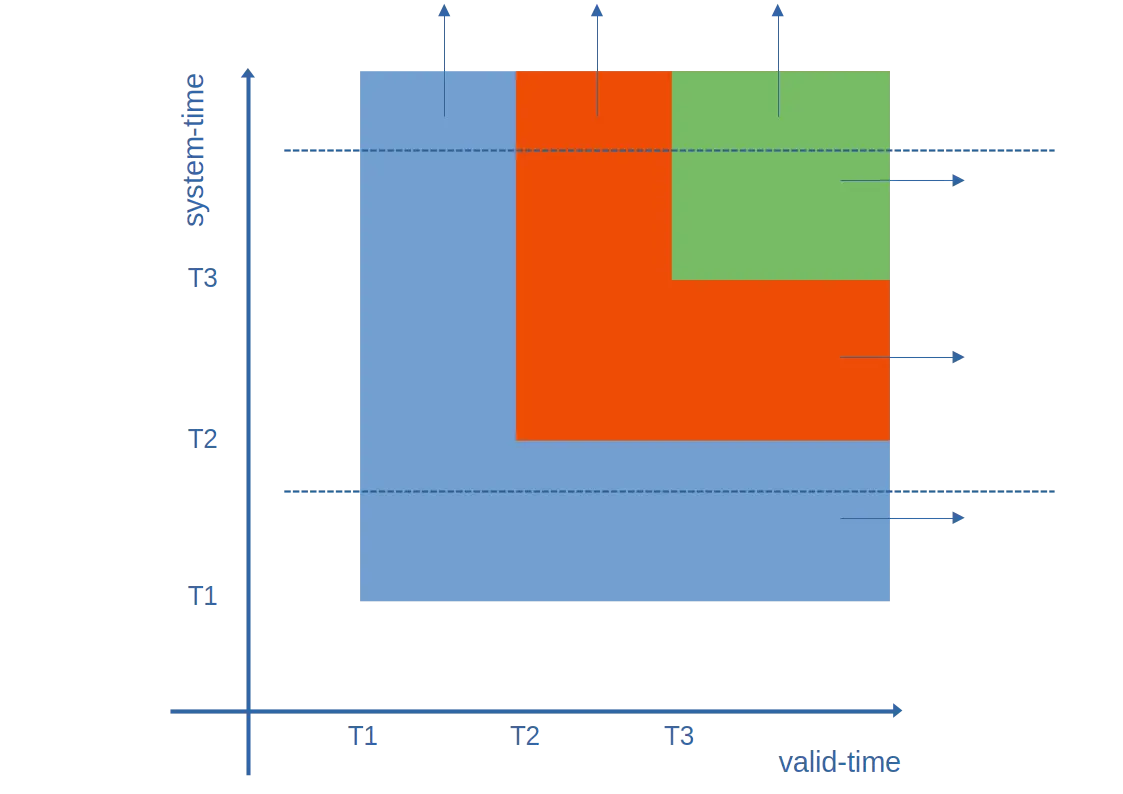
In this diagram:
-
The first version is in blue. It’s then superseded by orange, and again by green.
-
Taking a view of the timeline between T1 and T2 (bottom dashed line), we thought the entity would be forever blue - hence extending to the right-hand side.
-
Currently (top dashed line), and for all system-times into the future, we know that it was blue between T1 and T2 (valid time), orange between T2 and T3, and green from T3.
The events for this entity here are as follows:
| colour | system-from | valid-from | valid-to |
|---|---|---|---|
green |
T3 |
T3 |
∞ |
orange |
T2 |
T2 |
∞ |
blue |
T1 |
T1 |
∞ |
For the case of SELECT * FROM colours (i.e. as-of-now, by default), we play one event, yield green, and immediately skip to the next entity.
As the meerkat says, 'simples!'.
If we’re asked for FOR VALID_TIME AS OF <T2>, we still play through the events in reverse system time order - we ignore the green one, yield the orange one, and move on to the next entity.
The interesting cases start when we’re asked for the effective valid-from, valid-to, system-from or system-to of the rows - this is where the 'resolution' comes in. This time, when we’re playing through, we keep track of (what we call) the 'system-time ceiling' as we go - "for each segment of the valid-time timeline, at what point in system-time will earlier events get superseded?".
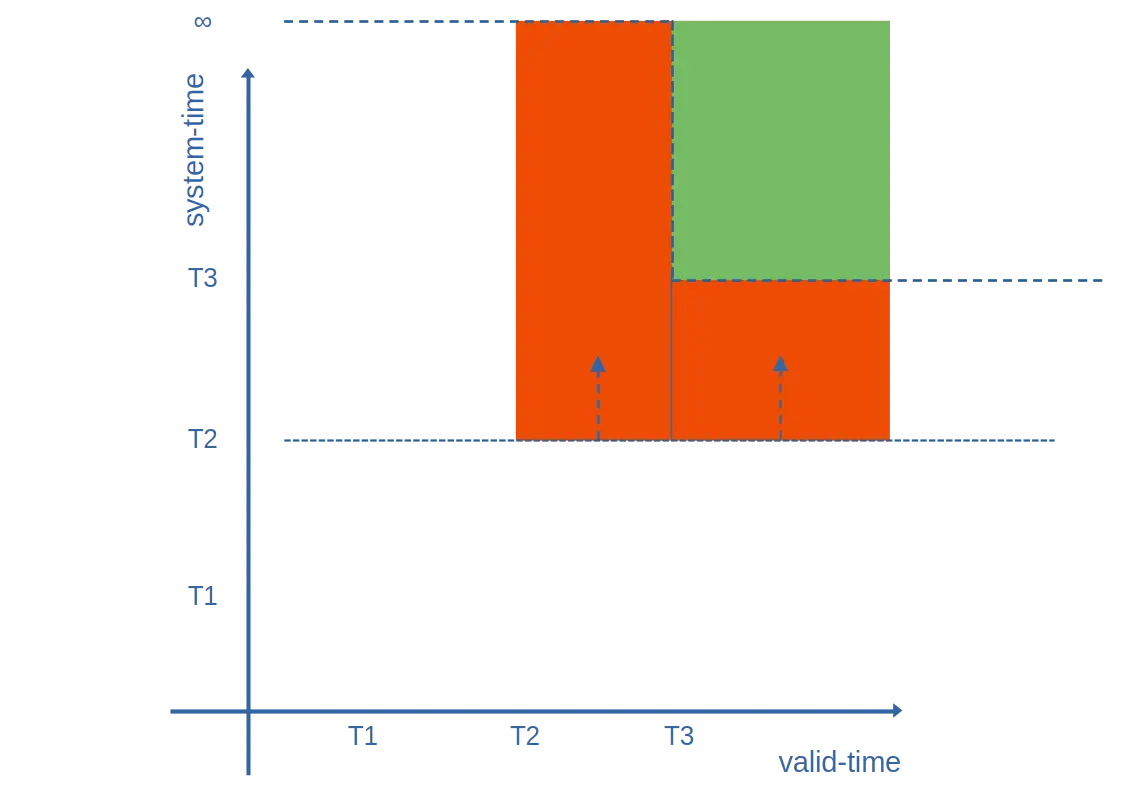
Best explained with a diagram (and hopefully you’ll see why we called it a 'ceiling' 😄):
-
The ceiling is initialised to "for valid-time from -∞ → ∞, ceiling = ∞"
-
After we play the green event, we lower the ceiling from valid-time T3 → ∞ to system-time T3
-
When playing the orange event (valid-time T2 → ∞ from system-time T2), we look up at the ceiling from the system-time = T2 line, creating two rectangles: valid T2 → T3 for system-time T2 → ∞, and valid T3 → ∞ for system-time T2 → T3.
-
We then lower the ceiling again, and play the blue event.
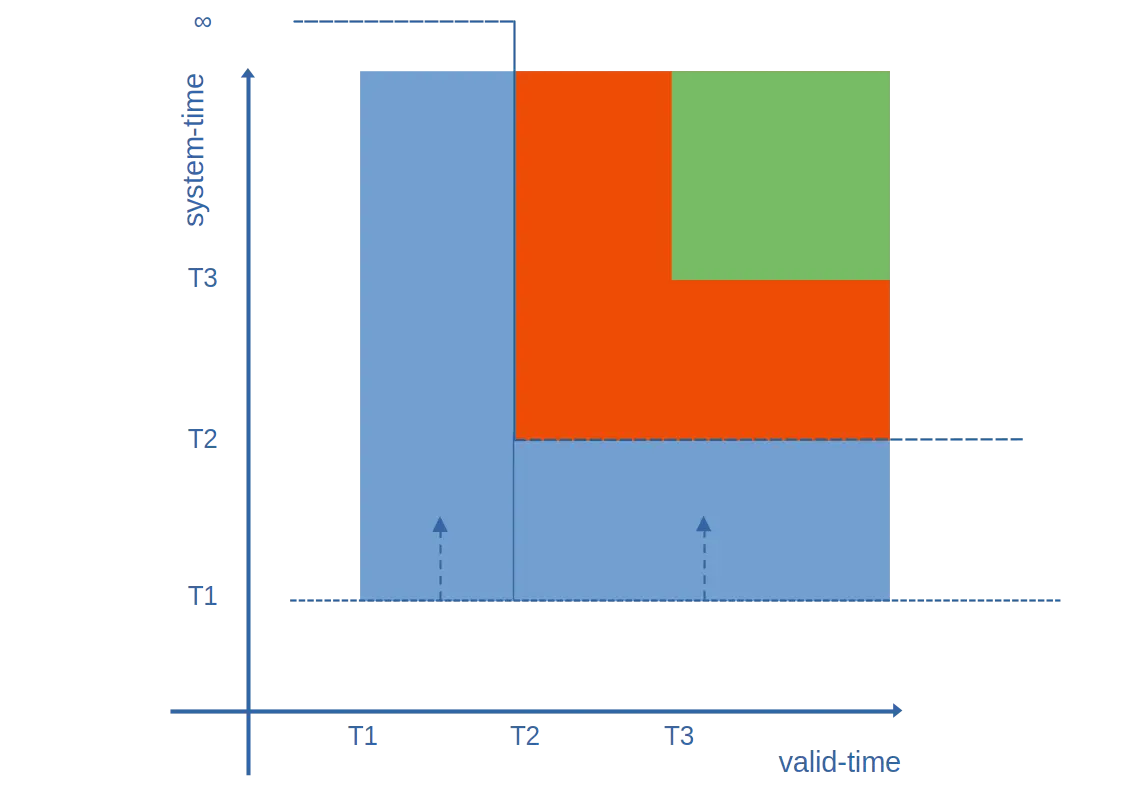
Working through the example, we get the following ceiling polygons and rectangles (see if you can spot them on the diagram):
| event | ceiling before | calculate rectangles | ceiling after |
|---|---|---|---|
green |
-∞ → ∞: ∞ |
valid: T3 → ∞; system: T3 → ∞ |
-∞ → T3: ∞ T3 → ∞: T3 |
orange |
-∞ → T3: ∞ T3 → ∞: T3 |
valid: T2 → T3; system: T2 → ∞ valid: T3 → ∞; system: T2 → T3 |
-∞ → T2: ∞ T2 → ∞: T2 |
blue |
-∞ → T2: ∞ T2 → ∞: T2 |
valid: T1 → T2; system: T1 → ∞ valid: T2 → ∞; system: T1 → T2 |
-∞ → T1: ∞ T1 → ∞: T1 |
Those rectangles then yield the following rows:
| colour | valid-from | valid-to | system-from | system-to |
|---|---|---|---|---|
green |
T3 |
∞ |
T3 |
∞ |
orange |
T2 |
T3 |
T2 |
∞ |
orange |
T3 |
∞ |
T2 |
T3 |
blue |
T1 |
T2 |
T1 |
∞ |
blue |
T2 |
∞ |
T1 |
T2 |
Sorted!
Now all we have to do is whatever joining/filtering/projecting/grouping/sorting the user’s requested in the rest of the query. 😅
Enter the time-series data:
The above pattern, roughly speaking, applies to most stateful entities. With the exception of back-in-time corrections or forward-in-time scheduled updates (which are usually relatively few in number compared to 'normal' events), we can assume that most events follow the pattern of 'with effect from valid-time now until their next update'. This means that the ceilings in the examples above stay a relatively small, constant size (2 entries, in the most common case) - and maybe you can now start to see our initial (flawed) assumption when we introduce time-series data…
When representing IoT device reading data in XT, say, we recommend modelling each device using a single entity; each reading using a small valid-time period for which that reading was valid - this allows you to use the valid-time timeline of that entity to see the reading history.
For example, let’s say you’re monitoring the wind speed at various locations. If you receive readings like "from 12:00 to 12:05 the average speed at location X was 12km/h", "from 12:05 to 12:10 the average speed at X was 14km/h", you’d represent it with two inserts as follows:
INSERT INTO wind_speeds (_id, _valid_from, _valid_to, wind_speed)
  VALUES ('X', TIMESTAMP '2024-07-16T12:00Z', TIMESTAMP '2024-07-16T12:05Z', 12.0);

INSERT INTO wind_speeds (_id, _valid_from, _valid_to, wind_speed)
  VALUES ('X', TIMESTAMP '2024-07-16T12:05Z', TIMESTAMP '2024-07-16T12:10Z', 14.0);

-- let's have one at location Y, too, for good measure
INSERT INTO wind_speeds (_id, _valid_from, _valid_to, wind_speed)
  VALUES ('Y', TIMESTAMP '2024-07-16T12:00Z', TIMESTAMP '2024-07-16T12:05Z', 18.5);
You’d then be able to query it using FOR VALID_TIME … - e.g.:
-- give me the whole history of location X
SELECT *, _valid_from, _valid_to
FROM wind_speeds
  FOR ALL VALID_TIME
WHERE _id = 'X';

-- give me the wind-speeds at all locations between 12:00 and 12:10
SELECT *, _valid_from, _valid_to
FROM wind_speeds
  FOR VALID_TIME
FROM TIMESTAMP '2024-07-16T12:00Z' TO TIMESTAMP '2024-07-16T12:10Z'However…
Let’s say over the course of a few months we have tens of thousands of such readings for each entity. [2]
What does the ceiling look like?
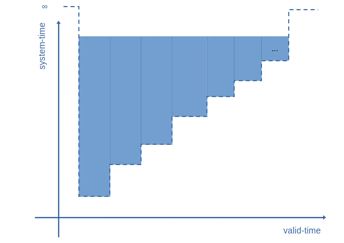
Uh oh!
Looks like one entry in the ceiling for every version, because none of the versions are bringing the ceiling down outside of their own valid time range - i.e. the size of the ceiling polygon is O(n):
| event time | ceiling before | calculate rectangles | ceiling after |
|---|---|---|---|
valid T2 → T3; system T3 |
valid: T3 → T4; system: T4 → ∞ valid: T4 → T5; system: T5 → ∞ … |
T2 → T3; system T3 → ∞ |
valid: T2 → T3; system: T3 → ∞ valid: T3 → T4; system: T4 → ∞ valid: T4 → T5; system: T5 → ∞ … |
valid T1 → T2; system T2 |
valid: T2 → T3; system: T3 → ∞ valid: T3 → T4; system: T4 → ∞ valid: T4 → T5; system: T5 → ∞ … |
T1 → T2; system T2 → ∞ |
valid: T1 → T2; system: T2 → ∞ valid: T2 → T3; system: T3 → ∞ valid: T3 → T4; system: T4 → ∞ valid: T4 → T5; system: T5 → ∞ … |
If you’re doing operations (as we were) involving the whole ceiling for every event, while perfectly acceptable when the ceilings are a small, constant size,[3] in these circumstances it yields a not-so-cool O(n²) algorithm in the number of 'visible' versions of the entity.
Ouch!
Thankfully though, devoted readers who’ve made it this far, our story has a happy ending.
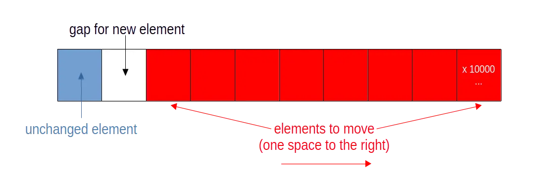
As you can see from the table above, in practice, our main operations for each event involved manipulating the start of the ceiling polygon array - inserting some values, deleting others.
However, inserting into/deleting towards the start of a large array is very costly - you need to copy all of the subsequent elements (most of the array) one place to the right/left [4] - hence the ~O(n) operation for each event.
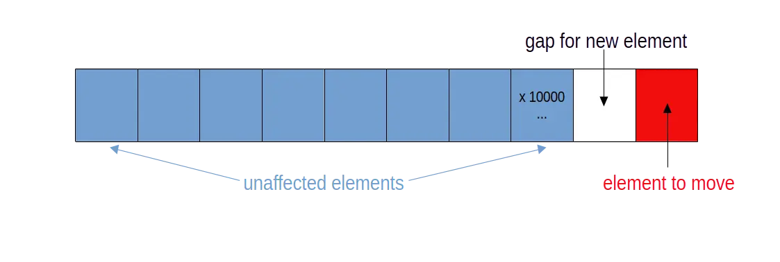
Our fix, in this case, was to reverse the order of the array, so that the manipulations we were making were instead towards the end of the array. Because inserting/deleting elements here only involves moving a small number of elements, this means that our insertions and deletions are now back to O(1), and the overall operation back to O(n).
Safe to say, a very satisfying fix 😊
Until next time!
James