Fraud detection with XTDB

Fraud detection often means making decisions before all the facts are available. A payment needs a fraud-risk score now, but confirmation that an earlier transaction was fraudulent may arrive weeks later. Account details and transaction records can also be corrected after a decision has been made.

Using a model to detect fraud requires two stages: training and serving.

• Training uses historical transactions, labelled as fraudulent or legitimate, to build a model that estimates the probability of fraud. Its inputs must reflect the information available when each transaction was scored.
• Serving uses the model produced by training to score new transactions. For each transaction, we calculate the model’s inputs, called features, such as recent spending and previously confirmed frauds, and pass their values to the trained model.

Keeping these calculations consistent matters. If training uses information that serving would not have had, the model can appear more accurate than it will be in production.

The team responsible for the model must also be able to explain its decisions. For audit purposes, we need to:

• Reconstruct a decision: recover the inputs, model version and score used to approve, decline or flag a transaction.
• Reproduce the training dataset: recover the dataset used to train a particular model, including what was known at each historical decision.
• Trace the impact of corrections: establish what changed, when it was recorded, and whether it would alter an earlier score.

XTDB is a good fit for these requirements for two reasons:

• One data store for training and serving. Both use the same underlying records, reducing the need to copy data between stores and keep those copies consistent.
• Queries against historical database states. XTDB lets us query the database as it stood at a chosen point in time, so later confirmations and corrections do not prevent us from reproducing earlier results.

This post follows a small fraud detection system built on XTDB, with 50,000 generated card transactions across 150 accounts.

Training needs feature values for many historical transactions; serving needs them for one transaction as it arrives.

A feature store manages these values for both uses. An offline store supports bulk training, while an online store provides fast lookups for serving. Keeping the two consistent requires updates to reach both.

The demo computes features directly from the same XTDB tables for training and serving. A new fraud confirmation is available to the next query without copying it into a separate feature store.

The model

A transaction’s fraud risk depends on the account’s activity as well as the payment itself. The demo uses four features to capture that context, combining them through logistic regression to estimate the probability of fraud:

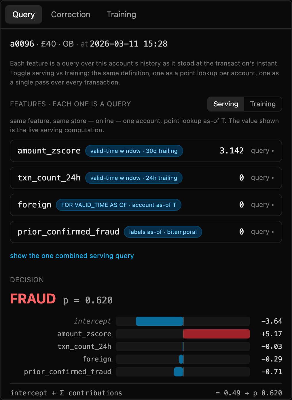
• amount_zscore: how far the amount is from the account’s usual spend over the previous 30 days
• txn_count_24h: how many transactions the account made in the previous 24 hours
• foreign: whether the transaction’s country differs from the account’s home country
• prior_confirmed_fraud: how many of the account’s transactions in the previous 90 days have been confirmed as fraud

For training, each transaction also needs a label: whether it was fraudulent. That outcome may become known only after an investigation. Training pairs the inputs available at the decision with the eventual outcome, producing a model that can score new transactions.

Training the model

Each historical transaction becomes a training example: four feature values paired with its eventual fraud outcome. We build these examples by combining transactions from txn, account attributes from account and classifications from label. Each transaction has an event time, txn_ts, and its classification history is linked by the same transaction ID.

The demo trains only on transactions at least 30 days old, the maximum delay for a fraud confirmation in the simulation. It fits the model to the resulting dataset and saves the trained model together with its evaluation metrics. We can rerun the training queries as new transactions and confirmations become available, then train and evaluate an updated model.

The queries calculate spending and transaction counts over windows preceding each transaction. They exclude the transaction itself from its own history and read the account attributes that applied at that time. The prior-fraud feature also needs to account for when earlier frauds were confirmed.

Late fraud confirmations

Suppose a stolen card is used on 5 March and another transaction on the same account is scored on 20 March. The investigation confirms the 5 March fraud on 25 March, and the disputed payment is reversed through a chargeback. A training query run in late April must exclude that confirmation from the 20 March transaction’s input features: it was unavailable when the transaction was scored.

Using today’s fraud classifications for every historical transaction would include such later confirmations. A model trained and tested on those inputs could learn to rely on information unavailable in production, overstating its accuracy. Retrieving the inputs available at each historical decision is known as point-in-time correctness.

To build these training examples, we need the classification available at each decision. To reproduce the dataset later, we also need the history as it was recorded when we ran the training query. XTDB represents these two timelines using valid time and system time. Valid time describes when the fact applies in the world; system time records when that version was present in the database. For the demo’s label table, valid time starts when a classification became available to the scoring system. The transaction’s event date remains in txn.txn_ts.

For the 5 March fraud, label.is_fraud becomes true from 25 March. Before then, the label records that the transaction had not been identified as fraud. The application supplies the availability time, and XTDB retains the label’s valid-time intervals and records subsequent changes in system time. The supplied history must reflect when the scoring system could actually use each classification.

If a confirmation became available to the scoring system on 25 March but was imported into XTDB on 27 March, its valid time would start on 25 March. A system-time query for 26 March would still show the database before that import.

Querying historical feature values

The same distinction applies to every transaction in the training dataset: which earlier frauds had already been confirmed when it was scored? The following query uses each transaction’s timestamp to select the relevant label history and calculate prior_confirmed_fraud. r is the transaction whose features we are calculating, f is an earlier transaction on the same account, and s is that earlier transaction’s label.

SELECT r._id,
       COUNT(s._id) AS as_known_then
FROM txn r
LEFT JOIN txn f
  ON f.account_id = r.account_id
 AND PERIOD(r.txn_ts - INTERVAL 'P90D', r.txn_ts) CONTAINS f.txn_ts
LEFT JOIN label FOR ALL VALID_TIME AS s
  ON s._id = f._id
 AND s._valid_time CONTAINS r.txn_ts
 AND s.is_fraud
GROUP BY r._id, r.txn_ts

The first join selects earlier transactions within 90 days, excluding the transaction being scored. The second selects each earlier transaction’s label at the scoring time and counts it only if it was already classified as fraud. FOR ALL VALID_TIME makes the label intervals available to the join; CONTAINS selects the interval containing each row’s scoring time. The query does not request all system-time versions. By default, the query reads the label history recorded in the database now. The section on reproducing results shows how to read an earlier database state.

On 20 March, the 5 March fraud contributes nothing to the prior-fraud count. From 25 March onwards, it contributes one, while it remains within the 90-day window. Each row supplies its own scoring time, allowing one SQL statement to reconstruct the relevant historical classification for every transaction.

The complete training queries in model.py return two prior-fraud counts:

• as_known_then counts earlier frauds already confirmed when the transaction was scored.
• with_hindsight counts earlier frauds using the fraud outcomes recorded now, including confirmations received after the transaction was scored.

Training uses as_known_then. Comparing it with with_hindsight shows which transactions would receive different feature values if we included later fraud confirmations.

Serving the model

When a transaction arrives, the scoring service queries its feature values and supplies them to the saved model. The model returns a probability of fraud.

For the prior-fraud feature, the serving query needs one account and one decision time. Here :account identifies the account and :t is the incoming transaction’s timestamp:

SELECT COUNT(*) AS prior_confirmed_fraud
FROM txn FOR VALID_TIME AS OF :t AS f
JOIN label l ON l._id = f._id
WHERE f.account_id = :account
  AND PERIOD(:t - INTERVAL 'P90D', :t) CONTAINS f.txn_ts
  AND l.is_fraud

The query reads the current labels of earlier transactions in the account’s 90-day window. At the time of a new decision, those are the classifications available to the scorer. The bulk training query instead selects the label interval containing each historical transaction’s scoring time.

Training calculates features for many historical transactions; serving calculates them for one incoming transaction. Both use the same tables and feature definitions, and the demo’s tests check that the two query forms produce matching values.

A later confirmation changes the features available for subsequent scores without retraining the model or refreshing stored feature values. It can also change the score if we reassess an earlier transaction using the updated labels. That reassessment answers what the model would say with today’s information. An investigation into the original decision requires the data and model used then.

Reproducing training data and decisions

The training and serving queries above read the history currently recorded in XTDB. To meet the audit requirements from the introduction, we also need to reproduce their results after that history changes. A system-time cutoff lets us read the database as it stood when the original query ran:

SETTING DEFAULT SYSTEM_TIME AS OF :as_of

This setting applies to every table in the query unless explicitly overridden. It reads the row versions present at :as_of and excludes later changes. Valid-time conditions still select the intervals required by the query, such as the label available at each training transaction’s scoring time.

Reproducing training data

Later confirmations or corrections can change the dataset returned by the same training query. Recording the query, its parameters and the database timestamp lets us recover the dataset used for a particular model. Rerunning that query with the same system-time cutoff reproduces the dataset from the retained history, even if the data has since been corrected.

Reproducing a decision

Suppose a payment is later reported as fraudulent and we need to explain why it was approved. Running today’s model against today’s data may produce a different answer. The investigation needs the transaction inputs, database timestamp and model version used for the original decision. The demo records trained-model versions in model_registry, with evaluation metrics and a path to the saved model. The original model and system-time cutoff let it repeat the scoring query and calculation after later confirmations arrive.

The recording follows a £24 transaction on account a0033. With 19 earlier transactions confirmed as fraud, the model estimates a 13.4% probability of fraud. After seven more transactions in the same 90-day window are confirmed as fraudulent, the count rises to 26 and the estimate to 43.7%. The transaction and model are unchanged.

Keeping the transaction time fixed and using the original system-time cutoff restores the count of 19 and reproduces the original estimate of 13.4%. Both the original score and the reassessment exclude transactions that happened after the transaction being scored. The system-time cutoff determines whether later confirmations of earlier transactions affect the score.

The same history also supports corrections beyond fraud labels. An account’s home country or a transaction amount might be revised after a decision. Writing a correction with the appropriate valid time preserves the earlier database version, so it remains available when reproducing the original result.

Run the demo

The code is in xtdb-demos/fraud-detection. Docker Compose runs XTDB, the Python API and the UI.

git clone https://github.com/xtdb/xtdb-demos
cd xtdb-demos/fraud-detection
docker compose up -d
./bin/seed.sh                 # replay 50k transactions in arrival order, then train

Open http://localhost:5173, pick a flagged account, and confirm its chargebacks. Compare the updated score with the score retrieved using the earlier system-time cutoff. The generated data and model are intended to demonstrate these database queries, rather than provide a production fraud detector.

To try XTDB with a smaller example, start with the SQL quickstart and explore how valid time and system time change query results.

If your data arrives late or gets revised, we’d like to hear how you handle that history today and where it causes problems. Contact us at hello@xtdb.com or join us on Discord.